A model of mass extinction by M. E. J. Newman

Author:M. E. J. Newman
Language: eng
Format: epub
Published: 1997-02-11T16:00:00+00:00

I n F I

J I I I

10"'" 10"'' 10"' 10"' 10"' 10"' 10"' 10"' 10"' 10"'

fraction of species killed s

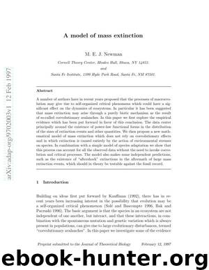
Fig. 6. The distribution of the sizes of extinction events during a simulation of the model described in Section 3. The distribution follows a power law closely over many decades, before flattening out around s = 10^^. In this example, in which the stresses on the system were drawn from a normal distribution, the power law has an exponent of 2.02 ± 0.02.

is no doubt that real species do interact and do coevolve. In Section 5 we will examine a more sophisticated variation of our model which reintroduces species interaction. However, the simple version presented here serves a very useful purpose, since as we will see, even without interaction between the species it reproduces all the forms of evidence for self-organized criticality put forward in Section 2, indicating that the mechanisms present here—stress-driven extinction, repopulation, and random uncorrelated evolution—are on their own perfectly adequate to explain the data.

4-1 Distribution of extinction sizes

The fundamental prediction of our model is that a certain number of species may be expected to become extinct at each time-step, and that the fraction s which does so depends on the level of stress placed on the system during that

18

step, and on the number of species present in the population whose abihty to withstand that stress is low. In Figure 6 we show a histogram of the sizes of the extinction events taking place over the course of a computer simulation of the model lasting ten million time-steps. The histogram is plotted on logarithmic scales, and the straight line form of the graph indicates that the histogram follows a power law of the form given in Equation (1). The only deviation is for very small extinction sizes, in this case below about one species in 10^, for which the distribution becomes fiat. However, extinctions this small are well below the noise level in our fossil data, so to the resolution of the data the prediction of our model is that the distribution of extinction sizes should be power-law in form. The distribution of applied stresses for the simulation shown in Figure 6 was normal with standard deviation a = 0.1 and mean zero:

Pstvessiv) OC exp

^2

2a'

(2)

The exponent r of the power-law distribution in Figure 6 can be measured with some accuracy and is found to be 2.02 ±0.02. Recall from Section 2 that the distribution of the sizes of extinction events in the fossil record has been found to be compatible with a power law form, and that this has been taken by some as an indication of self-organized critical behavior. Here, however, we see the same result emerging from a non-critical model of the extinction process, and furthermore, the measured value of r is in excellent agreement with the value of 2.0 ± 0.2 extracted from the fossil data.

In Figure 7, we show the distribution of extinction sizes for a wide variety of other stress distributions Pstrcss(^)- As

Download

Copyright Disclaimer:
This site does not store any files on its server. We only index and link to content provided by other sites. Please contact the content providers to delete copyright contents if any and email us, we'll remove relevant links or contents immediately.